Fig. 3.8.1: Fluctuations in the magnetic field strength (“total intensity”) as a result of the addition or reduction of the current and stored magnetic vectors

The measurement with the magnetometer, which is pulled behind the research ship at a distance of several hundred meters to one kilometer in order not to distort the sensitive measurement by the metal of the ship, which itself creates a magnetic field, shows the intensity of the magnetic field . The result is a curve that fluctuates more or less irregularly.

In Figure 3.8.1 you can see the measurement curve of a magnetometer that was towed behind a ship, drawn in blue. By far the largest proportion of the measured field strength, the so-called total intensity, is accounted for by the currently active Earth’s magnetic field. In our latitudes these are values ​​of around 45,000 nT (nano-Tesla). The fluctuations in the magnetometer measurements are much smaller and are in the range of a few hundred nT, but these cannot be explained by fluctuations in the intensity of the Earth’s magnetic field, because the value should actually remain the same everywhere. In fact, you can find the fluctuations that have turned out to be very important for plate tectonics.

These fluctuations reflect the magnetic information stored in the rocks of the ocean floor, with the polarity of the magnetic vector playing an important role. The magnetic vector of the current Earth’s magnetic field is the same everywhere, in this example it points to the south with an inclination of 45°, corresponding to the fact that the magnetic north pole is now in the south. The inclination value of 45° indicates that the measurement was taken at approximately 60° latitude. When the magnetometer is towed over the oceanic crust, it crosses areas of the oceanic crust of different ages and, depending on which polarity of the Earth’s magnetic field is stored in the section just passed over, the magnetic intensity is added if the magnetic paleovector and the current magnetic vector have the same magnetic polarity, and for reduction if they are opposite. This is shown in the small box in Fig. 3.8.1.

Fig. 3.8.2: Magnetometer measurements across a spreading zone with symmetrically arranged polarity changes (Meschede, unpubl. 2022).

The example of Fig. 3.8.2 shows a symmetrical section on both sides of a spreading zone. The magnetic stripe patterns arise parallel to the spreading zone and form stripes with varying polarities because the newly formed oceanic crust takes the stored information with it while driting away from the spreading center. And since spreading symmetrically produces new oceanic crust, correspondingly symmetrical stripe patterns emerge.

Fig. 3.8.3: Development of the magnetic stripe pattern (from Frisch & Meschede, 2021)

This principle of stripe pattern formation is shown in Fig. 3.8.3. Oceanic basalts with normal polarity were formed in the colored areas; the gray stripes show inverse polarity. In this way, the oceanic crust stores the temporal evolution of the stripes, because if one assumes that the spreading rate is constant over long periods of time, the formation age of the oceanic crust can be calculated from the distance of the stripes to the spreading zone.

Plate tectonics model spreading

Additional material: PDF file for download

The pdf file contains an easy to create paper/fabric model for developing the stripe pattern at a spreading zone.

The short video in Fig. 3.8.4 shows how the magnetic stripes are created by drifting away from the spreading center. The width of the respective strips depends on the frequency of the polarity reversals, which occur again and again, but not regularly, giving them a clear pattern that assigns them an age in connection with the neighboring strips based solely on their width. This works similar to a barcode that we all use almost every day at the checkouts in our supermarkets.

Fig. 3.8.4: Video animation for the development of magnetic stripe patterns (Meschede, unpubl., 2022)

Fig. 3.8.5: a) Magnetic stripe pattern on the Reykjanes Ridge south of Iceland (after Heirtzler et al.  1966), b) Curves of the magnetic field strength along the routes of ships crossing the spreading center of the Reykjanes Ridge (from Frisch & Meschede, 2021)

One of the first comprehensive magnetic surveys took place on the Reykjanes Ridge south of Iceland. In Fig. 3.8.5 you can see the individual curves of the measurement routes below, which were repeatedly driven across the spreading zone of the Reykjanes Ridge. The stripe pattern parallel to the spreading zone then results from many measurement curves lying next to one another. And if you correlate the measurement curves with the standardized magnetic time scale, you can determine the age.

Fig. 3.8.6: Dating of the magnetic stripe pattern by comparison with a standard magnetic profile (see Fig. 3.7.6 in Chapter 3.7), from Frisch & Meschede (2021)

Figure 3.8.6 shows an example of such an age determination. This is an excerpt from the investigation on the Reykjanes Ridge and here you can see how finely the age of the oceanic crust can be determined using magnetostratigraphy.

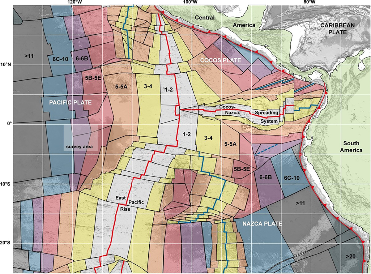
Fig. 3.8.7: Example of determining the age of the oceanic crust based on magnetic stripe patterns in the Pacific (modified after Meschede et al., 2008)

Figure 3.8.7 shows an example of how to age the entire oceanic crust using magnetic stripe patterns. And interesting connections are revealed, such as old, now deactivated spreading zones, which are shown in this figure by the blue lines. The currently active spreading zone in the Pacific is the East Pacific Ridge, shown here with the red line.

Such shifts in spreading zones happen again and again in the course of Earth’s history and it often happens that some branches are completely discontinued and new spreading zones open up. Ultimately, the plate movements react to all disturbances in the overall global movement pattern, because if a collision occurs somewhere on Earth, i.e. a plate movement is stopped, this has an impact on the entire plate pattern of the Earth.

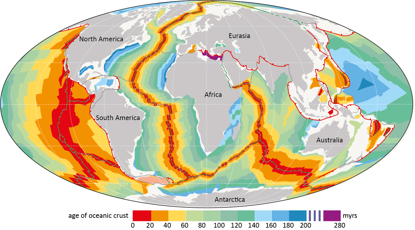
Fig. 3.8.8: Age of the oceanic crust (Meschede, unpublished, 2022, modified after Frisch & Meschede, 2021)

The magnetic stripe patterns are now known across the globe and this data has been used to create the map showing the ages of the oceanic crust in a global context (Fig. 3.8.8). One can immediately see that the spreading rate on the East Pacific Ridge was and is much higher than in the Atlantic. The strips are much wider in the Pacific than in the Atlantic, precisely because much more oceanic crust was formed there at the same time.